TiDB Computing

The previous article introduced how TiDB stores data. This is also the basic concept of TiKV. This article explains in detail how TiDB stores data in the lower-level Key-Value layer, maps the relational model to the Key-Value model, and executes SQL.

Mapping the Relational Model to the Key-Value Model

To simplify the relational model, consider only a simple table and SQL statements. What we need to think about is how table data is stored and how SQL statements are executed on Key-Value. Consider the following table.

CREATE TABLE User {...
    ID int,
    Name varchar(20),
    Role varchar(20),
    Age int,
    PRIMARY KEY (ID),
    Key idxAge (age)
};

Because the structures of a normal SQL database and Key-Value are very different, how to map an SQL database to Key-Value is important. First, to decide what kind of mapping solution is good, look at the characteristics of the data storage method.

A table contains three kinds of data. Metadata is not discussed here.

1. Metadata for the table
2. Number of rows in the table
3. Index data

Data can be stored by row or by column, and both have advantages and disadvantages. TiDB’s main purpose is online transaction processing, or OLTP, and it aims to quickly read, store, change, and delete data rows, so row storage is preferable.

TiDB supports both Primary Indexes and Secondary Indexes. Indexes are used for query acceleration, high query performance, and constraints. There are two query forms.

• Point query: finds a specific row of data through an index by using an equality condition such as a primary key or unique key, for example select name from user where id = 1;.
• Range query: for example, uses idxAge to query data where age is between 30 and 35, as in select name from user where age > 30 and age < 35;. There are two kinds of indexes, Unique Index and Non-unique Index, and TiDB supports both.

After analyzing the characteristics of the data to store, look at what is needed to manipulate data, such as Insert, Update, Delete, and Select statements.

• Insert statement: writes row data to Key-Value and creates index data.
• Update statement: changes row data and index data as needed.
• Delete statement: deletes both row data and indexes.
• Select statement: handles the most complex situations among the four.
  • Reads a row of data easily and quickly. In this case, each row needs an ID, explicit or implicit.
  • Reads several rows of data continuously, as in Select * from user;.
  • Loads data using indexes and uses indexes in point queries and range queries.

A globally distributed and ordered Key-Value engine satisfies the requirements above. The globally ordered characteristic helps solve many problems. Consider the following two examples.

• Fast lookup of data rows: assuming a single key or multiple keys can be created, TiKV’s Seek method can be used to quickly find the row.
• Full table scan: if a table can be mapped to a key range, all data can be retrieved by scanning from StartKey to EndKey. Index data can be handled in the same way.

Now look at how this works in TiDB.

TiDB assigns a TableID to each table, an IndexID to each index, and a RowID to each row. If a table has an integer primary key, that value is used as the RowID. TableID is unique across the entire cluster, and IndexID/RowID are unique within a table. All of these IDs are int64.

The data for each row is encoded as a key-value pair according to the following rule.

Key: tablePrefix{tableID}_recordPrefixSep{rowID}
Value: [col1, col2, col3, col4]

The tablePrefix/recordPrefixSep in the key are specific string constants and are used to distinguish different data in the Key-Value space. Index data is encoded as key-value pairs according to the following rule.

Key: tablePrefix{tableID}_indexPrefixSep{indexID}_indexedColumnsValue
Value: rowID

The encoding rule above applies to Unique Indexes, but a Unique Key cannot be created for Non-Unique Indexes because the index’s tablePrefix{tableID}_indexPrefixSep{indexID} is the same. Also, ColumnsValue can be the same across multiple rows. Therefore, some changes were made to encode Non-unique Indexes.

Key: tablePrefix{tableID}_indexPrefixSep{indexID}_indexedColumnsValue_rowID
Value: null

This method creates a unique key for each row of data.

In the rules above, all xxPrefix values in the key are string constants and serve to distinguish namespaces so that different kinds of data do not conflict.

var(
    tablePrefix     = []byte{'t'}
    recordPrefixSep = []byte("_r")
    indexPrefixSep  = []byte("_i")
)

Both row and index key encoding solutions have the same prefix. In particular, all rows of a table have the same prefix, and the data of an index also has the same prefix. Data with the same prefix is placed together in TiKV’s key space. Therefore, if the suffix encoding method is carefully designed so that the comparison relationship does not change, row or index data is stored neatly and in order in TiKV. The property that the comparison relationship does not change before and after encoding is called Memcomparable. For any value, the comparison result of two objects before encoding matches the comparison result of the byte arrays after encoding. Note that both keys and values in TiKV are primitive byte arrays. For details, see TiDB’s codec package. With this encoding method, all row data in a table is placed in TiKV’s key space according to RowID order. Data for a specific index is also placed according to the order of the index’s ColumnValue.

Now consider the requirements and TiDB’s mapping solution so far and confirm the feasibility of the solution.

1. First, the mapping solution converts row and index data into Key-Value data and ensures that each row and each piece of index data has a unique key.
2. It supports both point queries and range queries, so this mapping solution can easily create keys that correspond to part of a row or index.
3. Finally, when enforcing some table constraints, a specific key can be created and its existence checked to confirm whether the constraint is satisfied.

So far, this has explained how tables are mapped to Key-Value.

Next, consider another case with the same table structure. Suppose the table has three rows of data.

1, "TiDB", "SQL Layer", 10
2, "TiKV", "KV Engine", 20
3, "PD", "Manager", 30

First, each row of data is mapped to a Key-Value pair. This table has an integer primary key, so the primary key value is used as the RowID. Suppose the TableID of this table is 10 and the row data is as follows.

t10_r1 --> ["TiDB", "SQL Layer", 10].
t10_r2 --> ["TiKV", "KV Engine", 20].
t10_r3 --> ["PD", "Manager", 30].

This table has an index besides the primary key. Suppose the index ID is 1 and its data is as follows.

t10_i1_10_1 --> null
t10_i1_20_2 --> null
t10_i1_30_3 --> null

The encoding rules described above help explain this example. The goal is to understand why this mapping solution was chosen and what purpose it serves.

Metadata Management and SQL Implementation

The previous section explained the mapping between the relational model and the Key-Value model. This section introduces metadata management and how SQL is implemented.

Metadata Management

The previous section explained how table data and indexes are mapped to Key-Value. This section introduces how metadata is stored.

Both databases and tables have metadata that describes definitions and various properties. All this information must be stored in TiKV. Databases and tables each have a unique ID, and this ID becomes their unique identifier. When encoding as Key-Value, this ID is encoded with the prefix m_ in the key. The key is generated this way, and the serialized metadata is stored in the corresponding value.

In addition, a special Key-Value stores the current schema information version. TiDB adopts Google’s F1 online schema change algorithm. A background thread always checks whether the schema version stored in TiKV has changed. If there is a change, it manages the process so the change information can be received within a certain period.

Key-Value SQL Architecture

The following diagram shows TiDB’s overall architecture.

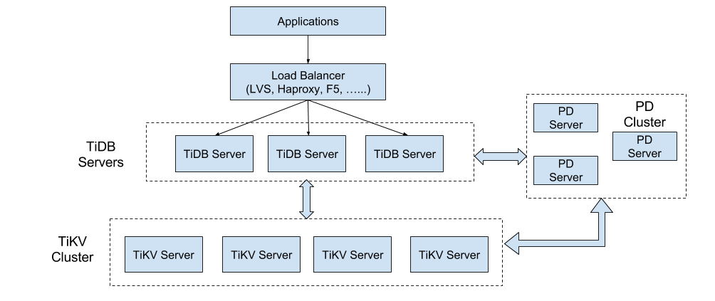
The main function of the TiKV cluster is a Key-Value engine that stores data, which was introduced earlier. This section focuses on the SQL layer, that is, TiDB Server. Nodes in this layer are stateless and do not store data, and each is exactly the same. TiDB Server is responsible for handling user requests and executing SQL operation logic.

SQL Computing

The mapping solution from SQL to Key-Value shows how relational data is stored. Next, it is necessary to understand how this data is used to satisfy query requests. In other words, this is the process by which query statements access data stored in the lowest layer.

The simplest method is to map SQL queries to Key-Value queries using the mapping solution introduced in the previous section and retrieve the corresponding data through the Key-Value interface before performing operations.

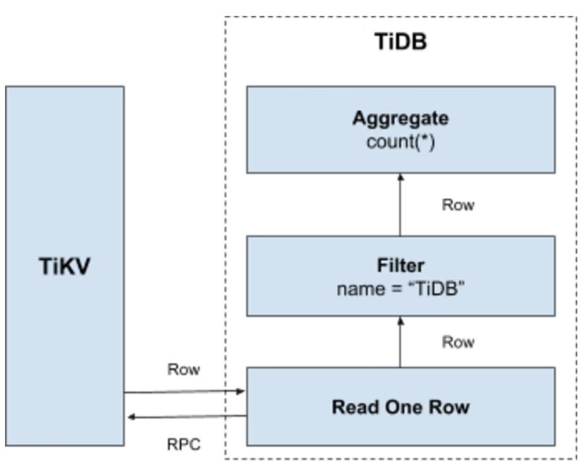
For the query Select count(*) from user where name= "TiDB";, all data in the table must be read and then checked to see whether the Name field is TiDB. If so, the row is returned. This operation is migrated to the following Key-Value operation process.

• Create key range: all RowIDs in the table are in the range [0, MaxInt64], so use 0, MaxInt64, and the row key encoding rule to create a left-closed and right-open interval such as [StartKey, EndKey].
• Scan key range: read TiKV data according to the key range created in advance.
• Filter data: when each row of data is read, evaluate the expression name = "TiDB". If the result is true, return this row. Otherwise, skip it.
• Count decision: for each row that satisfies the requirements, add to the Count value.

See the following diagram for the process.

This solution works, but it has the following disadvantages.

1. When scanning data, each row must be read from TiKV through a Key-Value operation. Therefore, at least one RPC overhead occurs. This overhead grows when a lot of data must be scanned.
2. It does not apply to all rows. Data that does not satisfy the condition does not need to be loaded.
3. The values of rows that satisfy the condition are not important. Only the row count is needed here.

Distributed SQL Operations

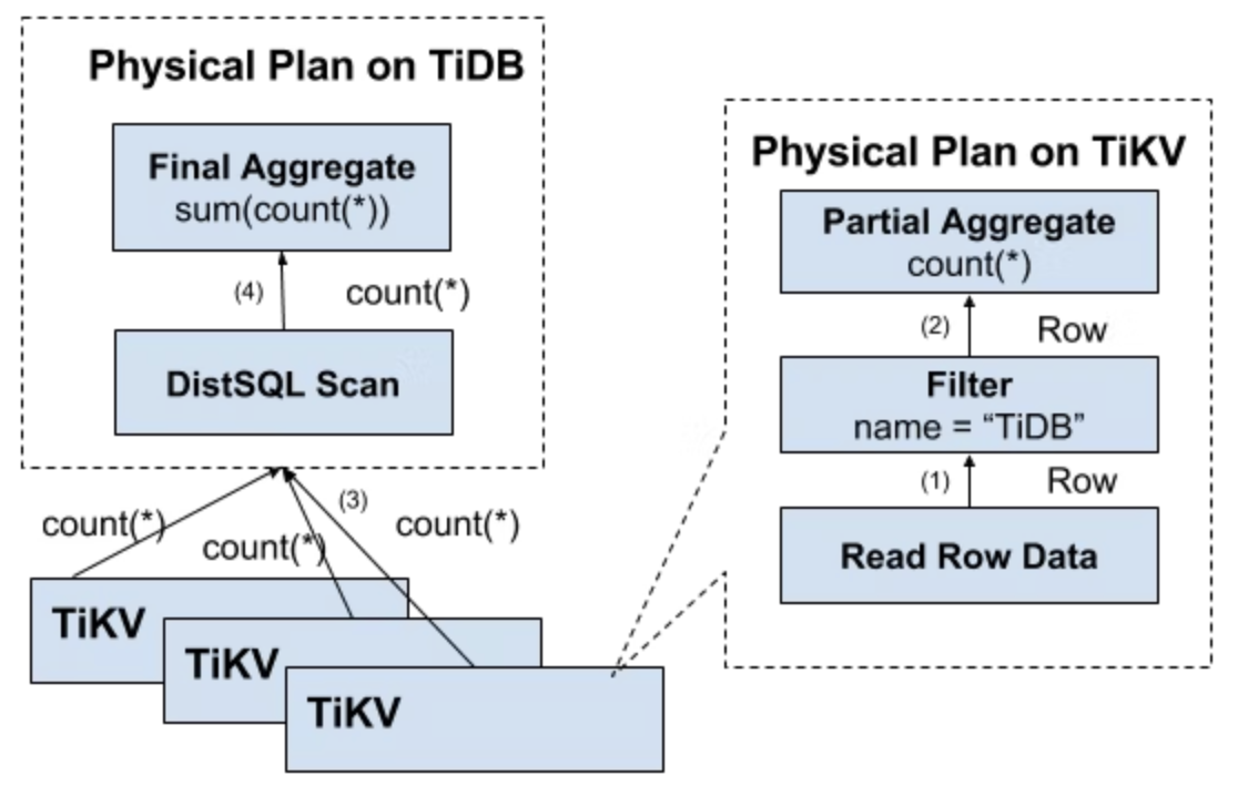
The disadvantages above can be avoided easily.

1. First, to stop a large number of RPC calls, work must be done close to the storage nodes.
2. Then, filters must be pushed down to the storage nodes. In this case, only valid rows are returned and meaningless network transmission can be avoided.
3. Finally, push down aggregate functions and GroupBy, and perform pre-aggregation. Each node can return only one Count value, and then tidb-server sums all values.

The following diagram shows data returning layer by layer.

SQL Layer Architecture

The previous sections introduced several functions of the SQL layer, so the basic concept of how SQL statements are processed should be clear. In fact, TiDB’s SQL layer is very complex and has many modules and layers. The following diagram shows all important modules and the relationships between calls.

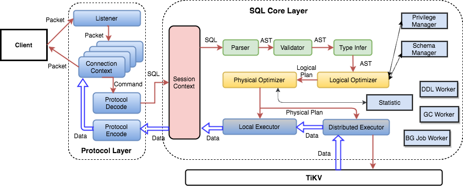
SQL requests are sent directly or through a load balancer to tidb-server. tidb-server parses MySQL protocol packets to identify the request content. It then performs parsing, creates and optimizes a query plan, executes the plan, and accesses and processes data. Because all data is stored in the TiKV cluster, tidb-server must interact with tikv-server to access data during processing. Finally, tidb-server returns the query result to the user.

Conclusion

This article introduced how data is stored and used for operations from an SQL perspective. Future articles will introduce information about the SQL layer, such as optimization principles and details of the distributed execution framework. The next article introduces PD, especially cluster management and scheduling.