Designing Data-Intensive Applications | Chapter 06. Partitioning

Presenters: Hyundo Park, Seungik Lee

Partitioning

If a dataset is very large or query throughput is very high, replication alone is not enough and the data must be split into partitions. This is called partitioning or sharding.

When partitions are created, each unit of data, such as a record, row, or document, usually belongs to one partition. A database may support operations that touch multiple partitions at once, but in practice each partition becomes a small database of its own.

In other words, a table remains one logical table, but physically it can be split into and managed as multiple tables.

Source: Real MySQL 8.0

Main Reasons for Partitioning

1. Scalability

• In a shared-nothing cluster, different partitions can be stored on different nodes. A large dataset can therefore be spread across multiple disks, and query load can be distributed across multiple processors.
• For queries that run on a single partition, each node can independently execute the query for its own partition, so query throughput can be increased by adding nodes. Large and complex queries are much harder, but they can still be executed in parallel across multiple nodes.

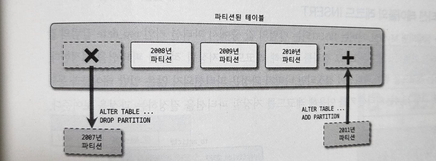
2. Efficient management of historical data

• Unnecessary data deletion work can be handled simply and quickly by adding or dropping partitions.
• Example: log data accumulates in large volumes over a short period, becomes useless after a certain period, and creates heavy load when deleted or backed up.

Partitioning and Replication

Replication and partitioning are usually applied together so that copies of each partition are stored on multiple nodes. Even though each record belongs to exactly one partition, it can be stored on several different nodes to ensure fault tolerance.

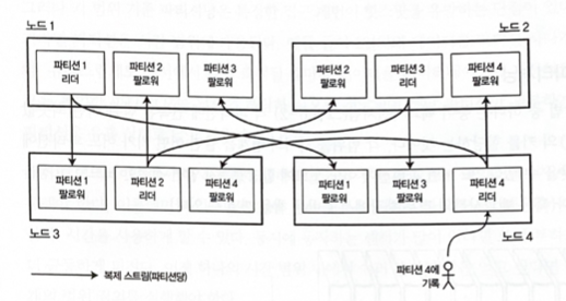
A single node may store multiple partitions. If the leader-follower replication model is used, the combination of partitioning and replication takes the following form.

The leader of each partition is assigned to one node, and followers are assigned to other nodes.

Each node can be the leader for some partitions and a follower for other partitions.

Partitioning Key-Value Data

• Skew: a situation where partitioning is not evenly distributed, so one partition has more data or receives more queries than other partitions.
• Hotspot: a term for a partition with disproportionately high load.

Partitioning by Key Range

This assigns a continuous range of keys to each partition. It allows the boundaries between ranges to be known and makes it easy to find which partition contains a given key. If you know which node each partition is assigned to, requests can be sent directly to the appropriate node.
Example: from a minimum value to a maximum value.

CREATE TABLE employees (
    id INT NOT NULL,
    first_name VARCHAR(30),
    last_name VARCHAR(30),
    reg_date DATE NOT NULL DEFAULT '1970-01-01',
    ....
) PARTITION BY RANGE( YEAR(hired) ) (
  PARTITION p0 VALUES LESS THAN (2000),
  PARTITION p1 VALUES LESS THAN (2010),
  PARTITION p2 VALUES LESS THAN (2020),
  PARTITION p3 VALUES LESS THAN MAXVALUE
);

Source: Real MySQL 8.0

Advantages

• Within each partition, keys can be stored in sorted order. This makes range scans easy and allows a key to be treated as a concatenated index, which can be used to read several related records with a single query.
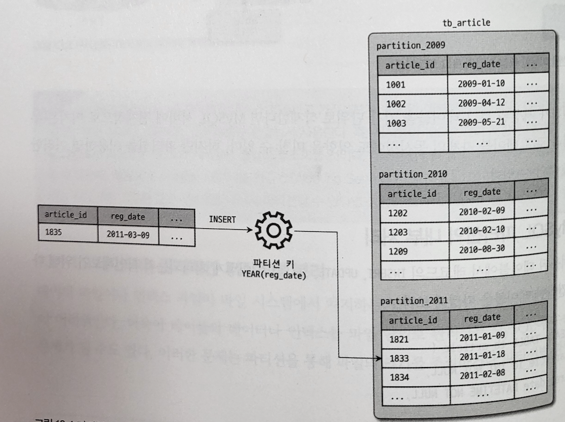
• Example: suppose an application uses the reg_date column of date type as a key. In this case, range scans are useful because all data for a specific year can be read easily.

Disadvantages

• Certain access patterns can create hotspots.
• If reg_date is the key, partitions correspond to year ranges. For example, one partition may handle one year’s data.
• Because every data update is written to the database, all writes can be sent to the same partition for the relevant year, overloading only that partition while the remaining partitions stay idle.

Partitioning by Hash of Key

Hash partitioning determines the partition in which a record is stored by using a specific hash function.

A hash function for partitioning does not need to be cryptographically strong. For example, Cassandra and MongoDB use MD5, and Voldemort uses the Fowler-Noll-Vo function. MySQL determines the target partition by dividing the result of an expression by the number of partitions and using the remainder.

Example: suppose there is a 32-bit hash function that takes a string as input. When a string is passed to the function, it returns a seemingly random number between 0 and 2^32 - 1. Even if input strings are almost identical, the hash values are uniformly distributed across the numeric range.

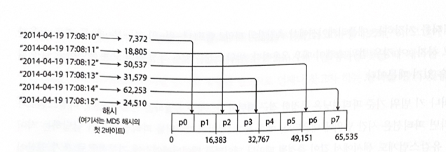
Figure 6-3. Partitioning by hash of key

Advantages

• It reduces the risk of skew and hotspots by taking skewed input data and distributing it uniformly.

Disadvantages

• It loses the useful property of key range partitioning that allows range queries to be executed efficiently.
• Keys that used to be adjacent are now scattered across all partitions, so sorted order is not preserved.
• In MongoDB, when hash-based sharding mode is enabled, range queries must be sent to all partitions. Riak, Couchbase, and Voldemort do not support range queries on the primary key.

Θ Cassandra
Cassandra compromises between two partitioning strategies. When declaring a table in Cassandra, you can specify a compound primary key that contains multiple columns.
Only the first part of the key is hashed and used to determine the partition, while the remaining columns are used as a concatenated index that sorts data in Cassandra’s SSTables.
In other words, you cannot use range queries on the first column of a compound key, but if you specify a fixed value for the first column, you can efficiently perform range scans on the other columns of the key.

Example: on a social media site, one user may upload several edited documents.

You can read all documents edited by a particular user in a given time interval, sorted by timestamp. Information edited by other users may be stored in different partitions, but information edited by one user is stored in timestamp order within one partition.
Primary key: (user_id, update_timestamp)

Skewed Workloads and Relieving Hotspots

As described above, choosing partitions by hashing keys helps reduce hotspots. However, it cannot eliminate hotspots completely. In the extreme case where the same key is always read and written, all requests are directed to the same partition.
Example: on a social media site, when a celebrity with millions of followers does something, it can cause a large reaction. That action may require writing a huge amount of data to the same key.
The key is probably the celebrity’s user ID or the ID of the action that people are commenting on. Since the hash value for the same ID is always the same, hashing does not help.

The solution suggested in the book:

• Add a random number to the beginning or end of each key. Even adding only two random decimal digits can evenly distribute writes for one key across 100 different keys, and those keys can be distributed across different partitions.
• However, if data is split across different keys, additional work is needed during reads. Data for 100 keys must be read and combined. Additional information must also be stored.
• This technique is reasonable only for a small number of hot keys. Applying it to most keys with low write throughput creates unnecessary overhead. Therefore, there must also be a way to track which keys have been split.

Partitioning and Secondary Indexes

If records are accessed only by primary key, the partition can be determined from the key and used to route read and write requests to the partition responsible for that key.
However, when secondary indexes, which are a way to search for items where a specific value occurs, are involved, things become more complicated.
The problem is that secondary indexes do not map neatly to partitions.

Partitioning Secondary Indexes by Document

An indexing method that handles only documents belonging to each partition and operates completely independently is called a local index.
When write operations such as adding, deleting, or updating documents are performed, only the partition containing the document ID to be written needs to be handled. It does not need to care what data is stored in other partitions.
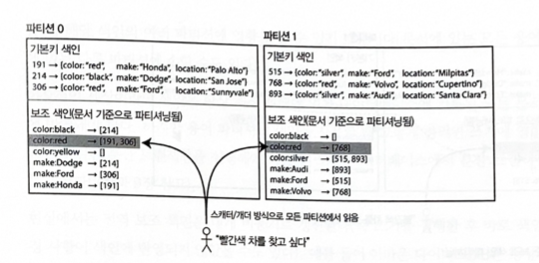
Example: suppose you operate a website that sells used cars. Each item has a unique ID called a Document ID, and the database is partitioned by document ID. Document IDs 0 to 499 are in partition 0, and Document IDs 500 to 999 are in partition 1.

Secondary indexes must be created on color and make. Once the indexes are declared, the database can automatically create index entries. For example, when a red car is added to the database, the database partition automatically adds it to the list of document IDs corresponding to the color:red index entry.

Cautions

• Unless special work is done on the document ID, there is no guarantee that cars of a specific color or manufacturer are stored in the same partition.
• In the image above, red cars exist in both partition 0 and partition 1.
• Therefore, if you want to find red cars, you must send the query to all partitions and collect all results.

This way of querying a partitioned database is also called scatter/gather. Queries that read using secondary indexes can be expensive.
Even if queries are executed in parallel across multiple partitions, scatter/gather is prone to tail-latency amplification. Nevertheless, secondary indexes are often partitioned by document.
Examples: MongoDB, Riak, Cassandra, Elasticsearch, SolrCloud, VoltDB.

In MySQL, indexes on partitioned tables are all local indexes. It does not support one globally integrated index for the whole table regardless of partitions.
Therefore, records matching the WHERE condition are read in sorted order and temporarily stored in a priority queue. Then the data is taken again from the priority queue in the required order.
As a result, when reading records through an index scan on a partitioned table, the MySQL server does not perform a separate sorting operation. It does not return results directly like an index scan on a normal table, and an internal queue-processing step is required.

Partitioning Secondary Indexes by Term

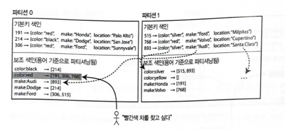
Unlike a local index, an index that covers data from all partitions is called a global index.
If such an index is stored on only one node, that node can become a bottleneck and defeat the purpose of partitioning, so the index is split across multiple nodes.

Because the partition of the index is determined by the term being searched, this type of index is called term-partitioned. Here, color:red is an example of a term.

Example: information about all red cars in all partitions is stored in the color:red entry of the index. The color index may be partitioned so that colors starting with letters from a to r are stored in partition 0, and colors starting with letters from s to z are stored in partition 1.

The car manufacturer index is partitioned in the same way.

Characteristics

• As before, indexes can be partitioned using the term itself or using the hash of the term. Partitioning by the term itself is useful for range scans, such as numeric attributes like the desired sale price of a car, while partitioning by the hash of the term distributes load more evenly.

Advantages

• Compared with document-partitioned indexes, the advantage of a global, term-partitioned index is efficient reads.
• A client does not need to perform scatter/gather across all partitions. It only sends the request to the partition that contains the desired term.

Disadvantages

• Writing a single document may affect several partitions of the index, making writes slow and complex.
• All terms in a document may belong to different partitions on different nodes.

Ideally, indexes are always up to date and every document written to the database is immediately reflected in the index.
However, doing this with term-partitioned indexes requires distributed transactions across all partitions affected by the write, and not every database supports distributed transactions.

In practice, global secondary indexes are usually updated asynchronously. In other words, if you read the index immediately after performing a write, the change may not yet be reflected in the index.
Example: Amazon DynamoDB usually updates global secondary indexes in less than one second under normal conditions, but if infrastructure failures occur, the propagation delay may become longer.

Other uses of global term-partitioned indexes include Riak’s search functionality and Oracle Data Warehouse. Oracle Data Warehouse lets you choose between local and global indexes.

Q. Local Index or Global Index? Which is easier to use?
A. It depends on the service structure and many other factors, but in general, because partitioned systems often perform operations such as add and delete on a specific partition, local indexes are used frequently because only the index of the target partition is affected. Global indexes create more load because operations involving a partition require overall readjustment.

Rebalancing Partitions

Overview Changes can occur in the physical machines of a database:

• CPU, RAM, or disk can be added.
• A new node can be added.

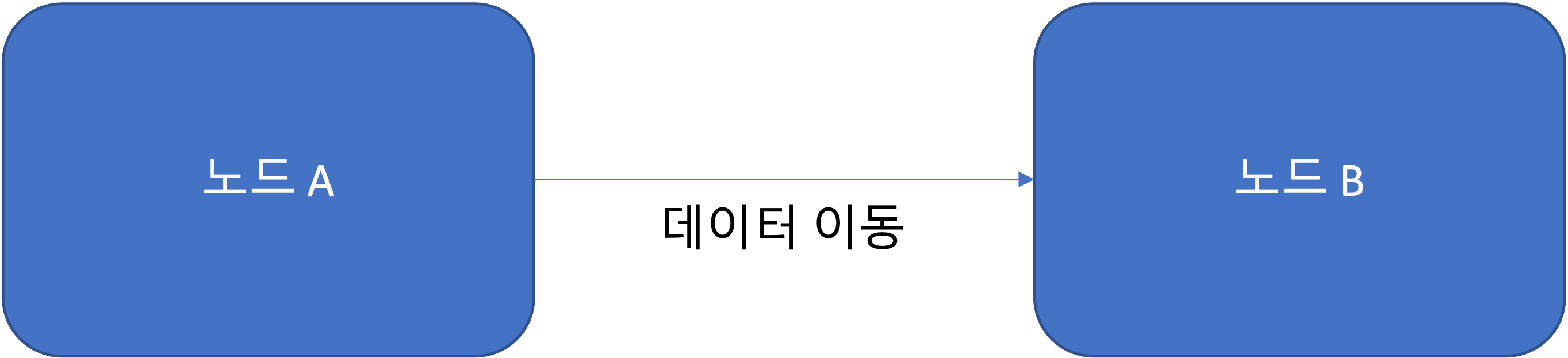
Rebalancing

• The process of moving load handled by one node in a cluster to another node.

Rebalancing requirements

• Even load distribution
• No service interruption
• Minimum data movement

Rebalancing Strategies

Hash value mod N, where N is the number of nodes

Problem with the mod N approach

• If the number of nodes N changes, most keys must be moved between nodes, increasing rebalancing cost.

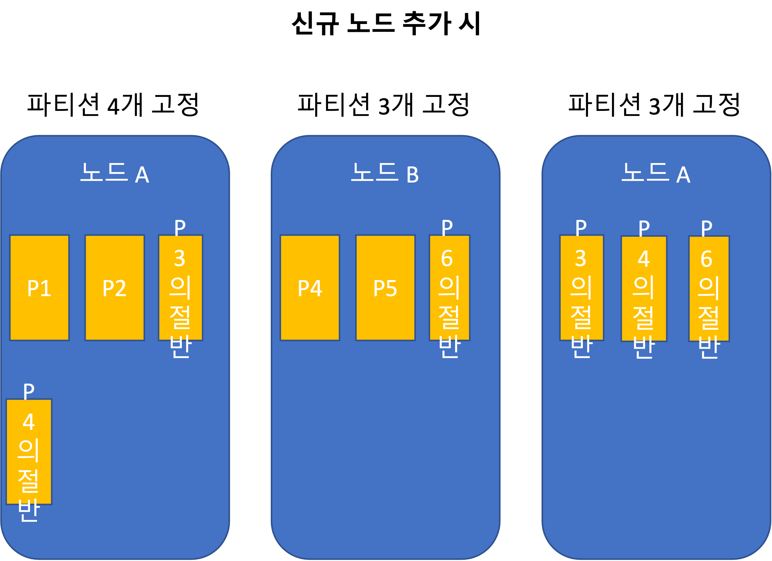
Static partitioning (fixed number of partitions)

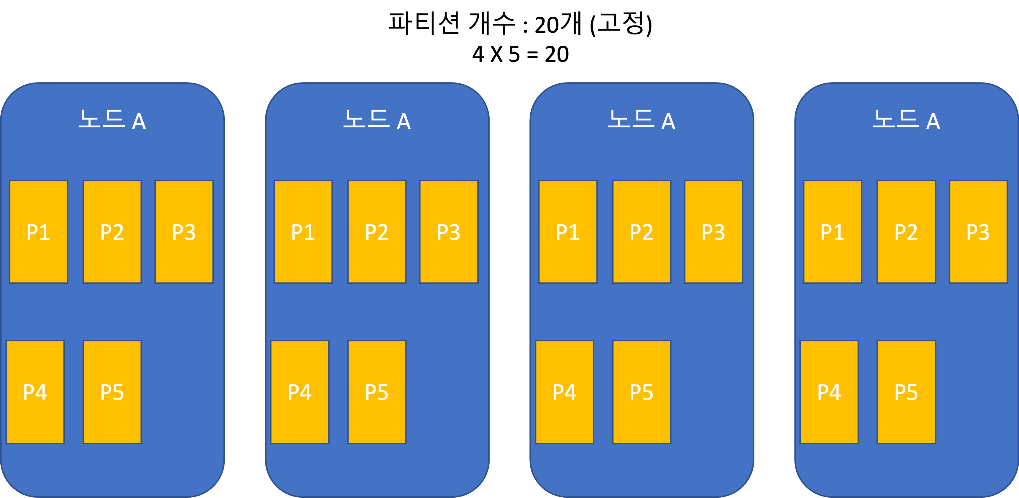
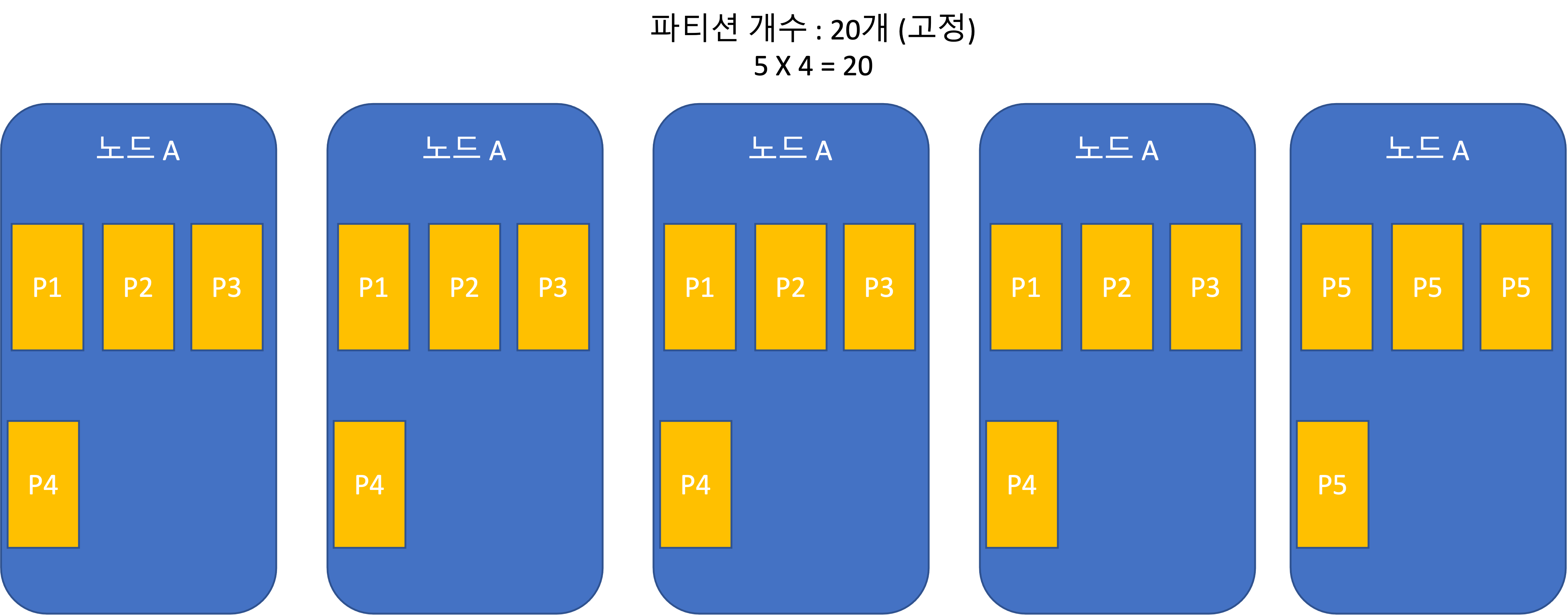
• Used by Riak, Elasticsearch, Couchbase, and Voldemort.
• If the total dataset size changes significantly, it is difficult to choose an appropriate number of partitions.
• If partitions become too large, rebalancing and failure recovery become expensive.
• Choosing an appropriate size is best, but difficult.

Dynamic partitioning Listing development team > 06. Partitioning > dynamic partitioning 1.png

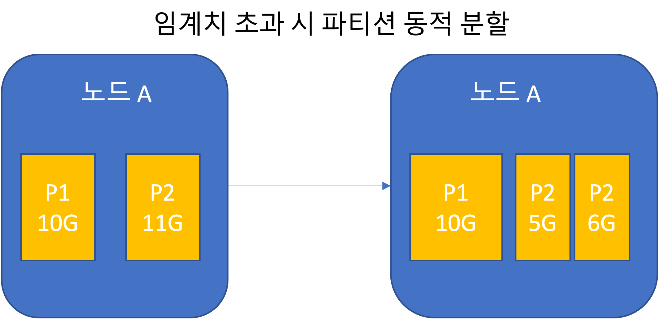
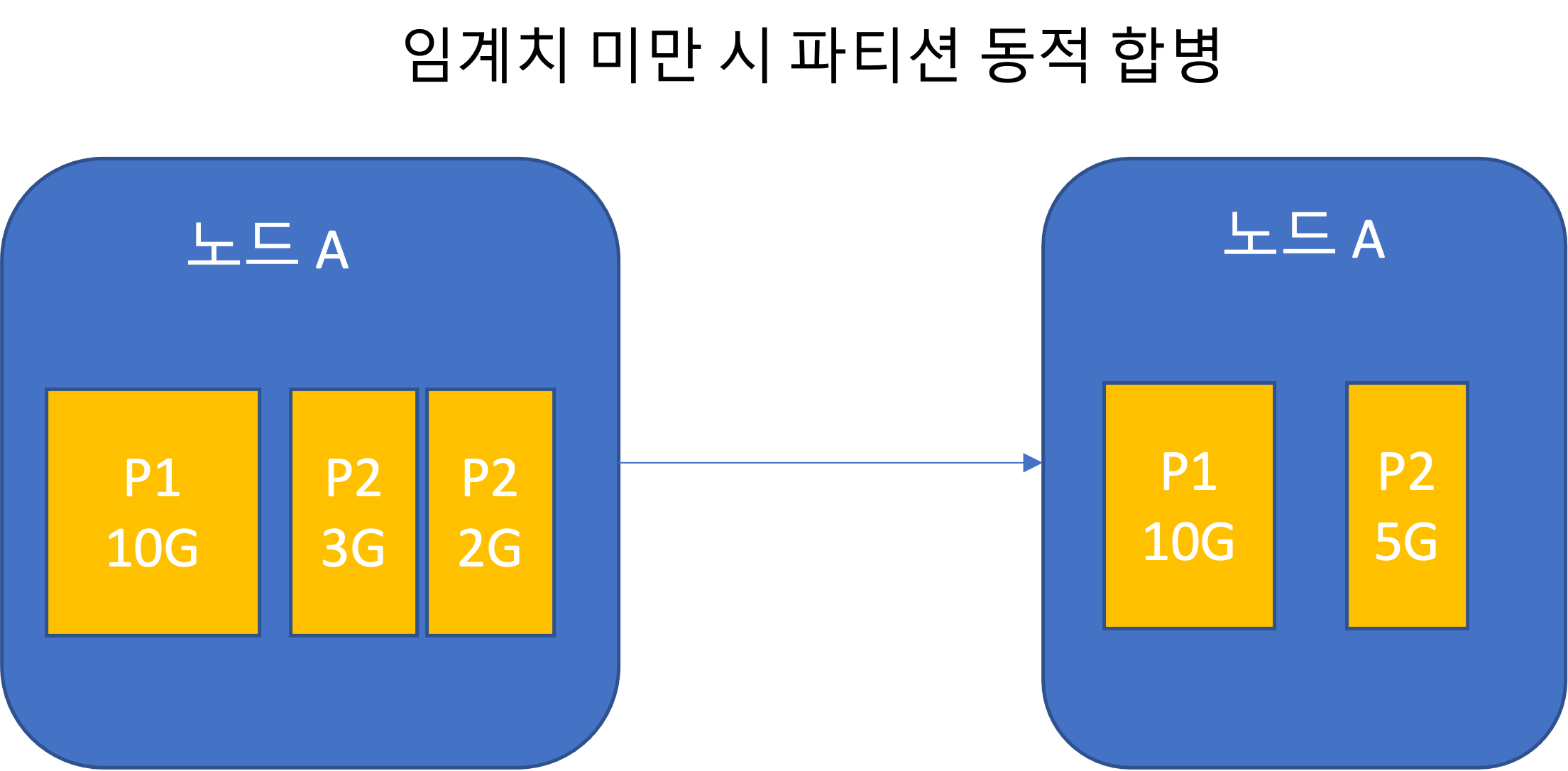
• The number of partitions is adjusted to match the total data volume by limiting size and increasing the count.
• In an empty database, there is only one partition until partition boundary settings are reached.
  • HBase and MongoDB can set an initial set of partitions for an empty database. This is called pre-splitting.

Summary of static and dynamic partitioning

• Static partitioning: partition size is proportional to data size.
• Dynamic partitioning: the number of partitions is proportional to data size.
• Neither approach is directly related to the number of nodes.

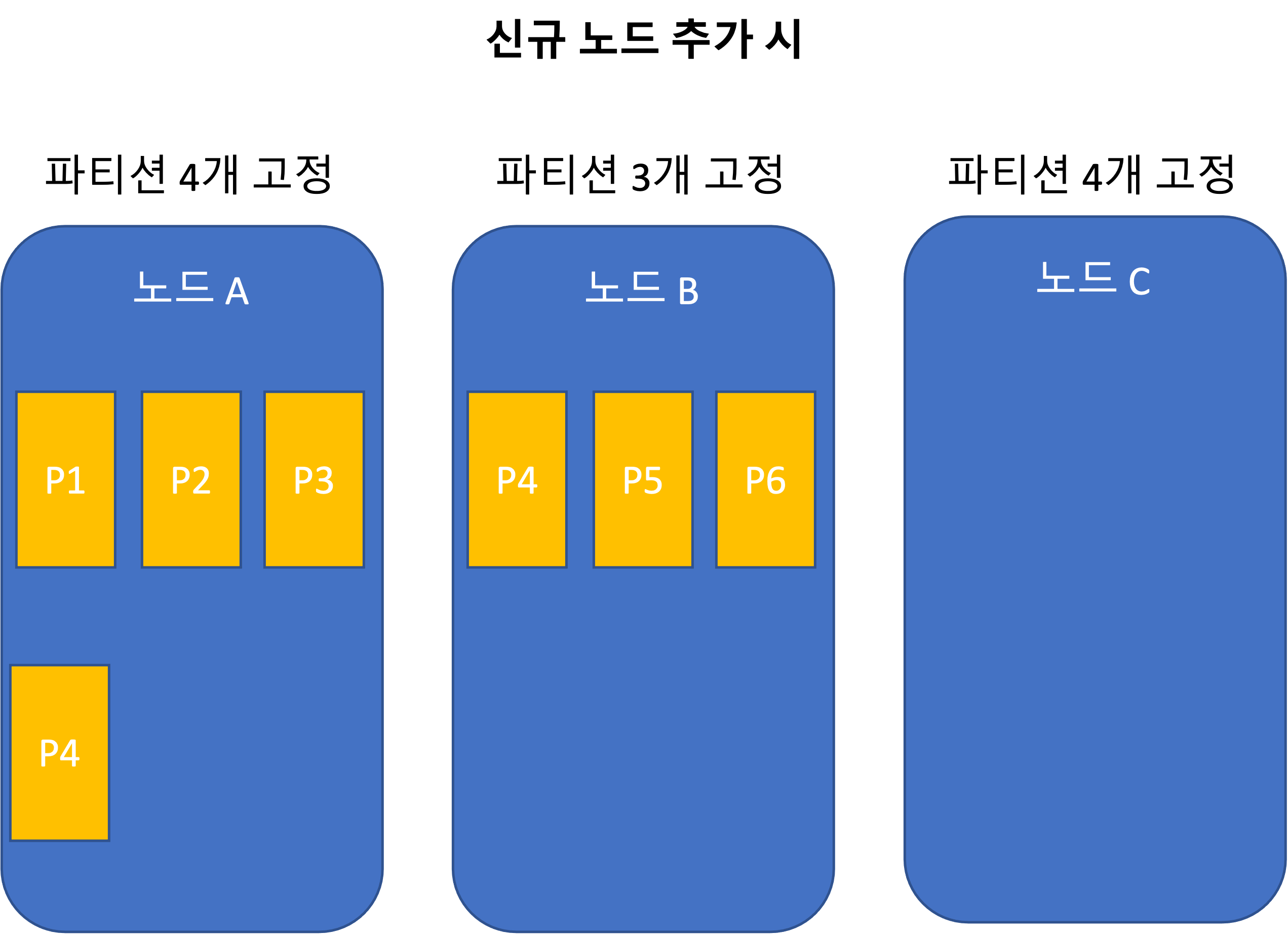
Node-proportional partitioning

Operations: Automatic and Manual Rebalancing

Fully automatic rebalancing

• The system rebalances automatically without any administrator intervention.

Fully manual rebalancing

• The administrator explicitly assigns partitions to nodes, and partition assignments change only when the administrator reconfigures them.

Request Routing

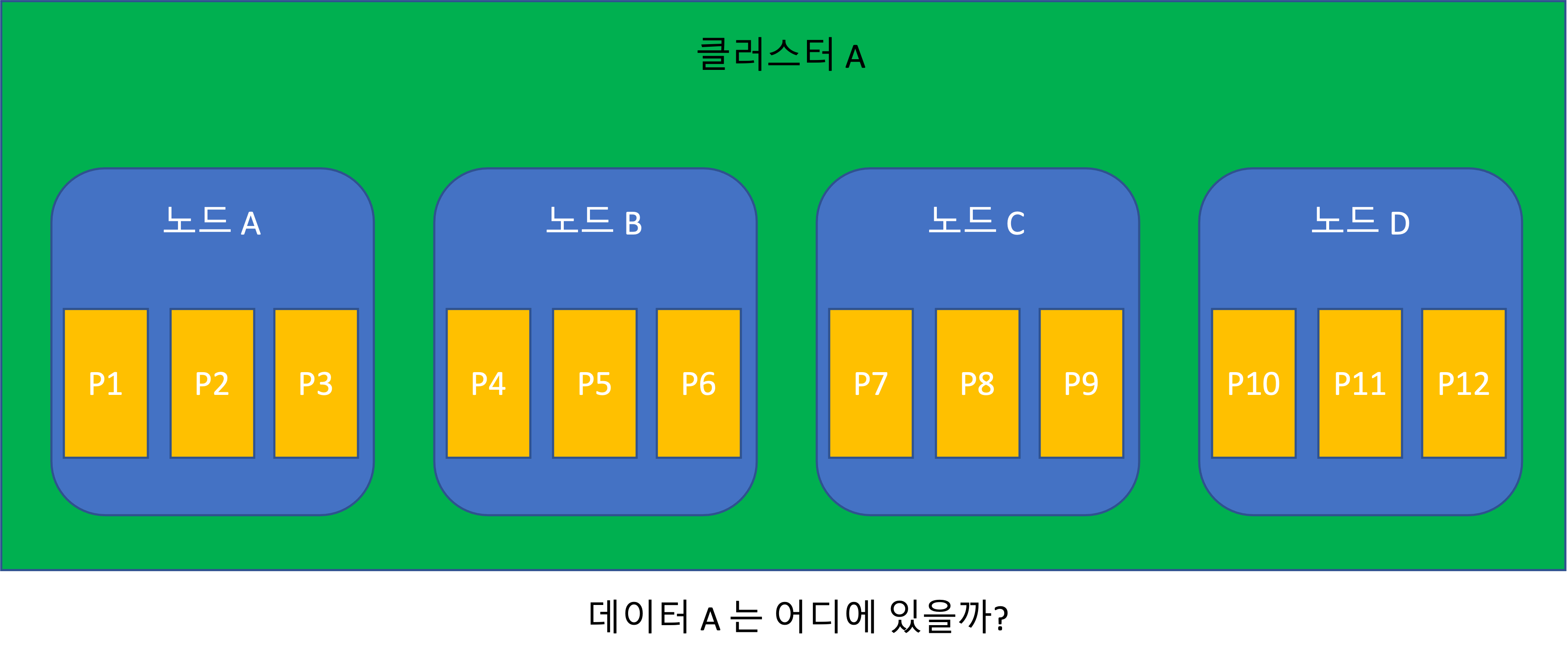
• As partitions are rebalanced, the partitions assigned to nodes change. This means the data locations change.
• This creates a requirement to keep track of partition assignment information in real time.

Service discovery

• A general problem not limited to databases.
• Any software aiming for high availability has this problem.
  • High availability effectively means a distributed network system.
• https://mangchhe.github.io/springcloud/2021/04/07/ServiceDiscoveryConcept

Approaches based on where the routing decision component is located Routing decision component? It means location information.

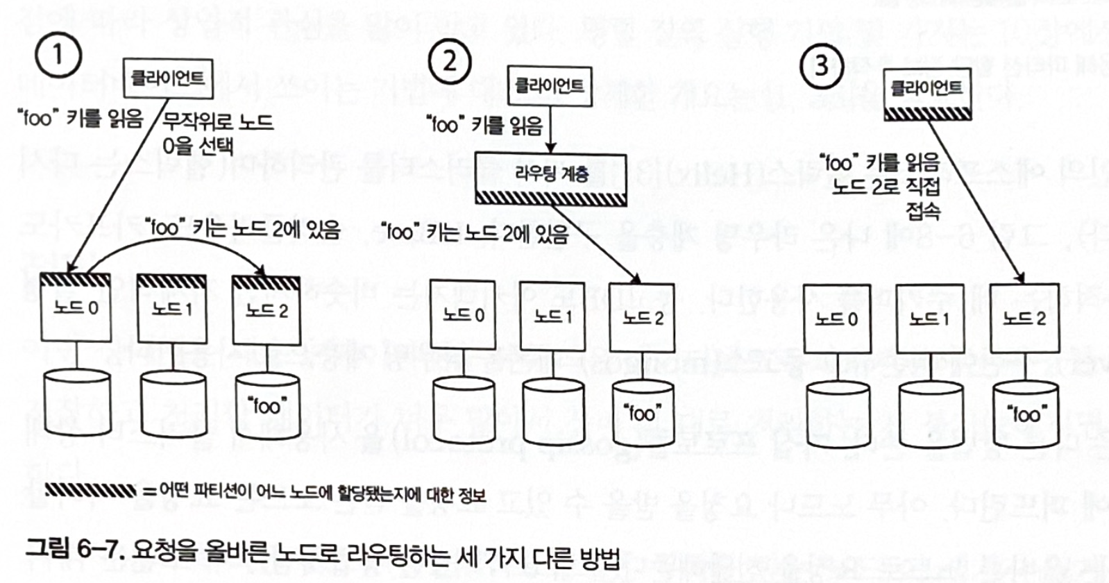
Figure 6-7. Three different ways to route a request to the right node

How to manage key information In every case, the key question is how the component making routing decisions can learn about changes to partition assignments on nodes.
Many coordination services exist: https://stackshare.io/service-discovery

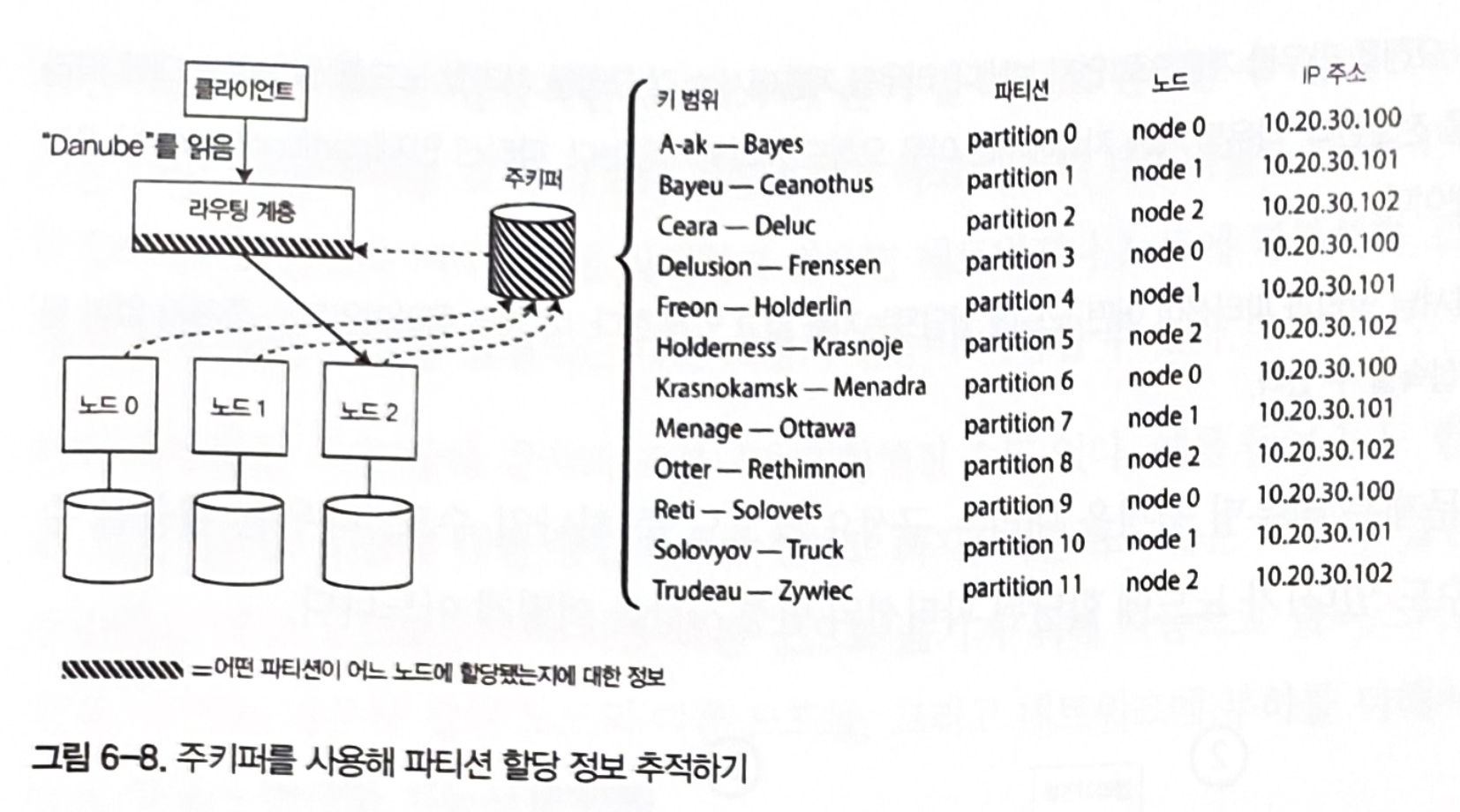
Figure 6-8. Tracking partition assignment information with ZooKeeper

How databases approach partition assignment information

Method 1. Each individual node owns partition assignment information.

• Cassandra, Riak
• This adds complexity to database nodes, but it has the advantage of not depending on an external coordination service.

Method 2. The routing layer owns partition assignment information.

• HBase, SolrCloud, Kafka, MongoDB
• Uses a coordination library or its own configuration server, as in MongoDB.

Method 3. The client owns partition assignment information.

• Please share examples.

Parallel Query Execution

• As data grows large, large-scale data analysis and querying become important, leading to clustered databases.
• Massively parallel processing, or MPP, is supported.
• RDBs support complex query types such as joins, filtering, grouping, and aggregation.
• MPP queries are executed in parallel on different nodes within a cluster.