Designing Data-Intensive Applications | Chapter 03. Storage and Retrieval

Presenters: Kyungcheol Kim, Mingyu Kim

This chapter looks at how databases store data and how they find it again when it is requested. To tune a storage engine for a particular workload, it helps to understand the work the engine performs internally.

The chapter compares two broad families of storage engines: log-structured engines and page-oriented engines such as B-trees.

Data Structures That Power Databases

The simplest key-value store can be implemented with two shell functions:

#!/bin/bash

db_set() {
    echo "$1, $2" >> database
}

db_get() {
    grep "^$1," database | sed -e "S/^$1,//" | tail -n 1
}

db_set appends a key and value to the end of a file. db_get scans the file and returns the most recent value for the requested key. Appends are fast, but lookups are slow because the whole file must be scanned. In algorithmic terms, lookup cost is O(n).

A database therefore needs an index: additional metadata derived from the primary data that helps locate records efficiently. Indexes speed up reads, but every index also slows down writes because the index must be updated whenever data changes. Choosing indexes is a trade-off based on the application’s query patterns.

Hash Indexes

A common key-value indexing strategy is to keep an in-memory hash map from each key to the byte offset of its latest value in the data file.

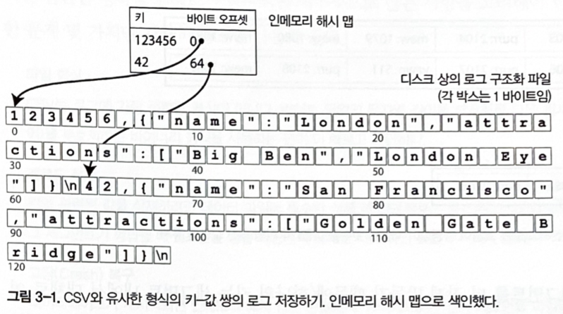
Figure 3-1. A log of key-value pairs in a CSV-like format, indexed with an in-memory hash map.

When a new key-value pair is appended, the hash map is updated with the newly written offset. On read, the engine looks up the key in memory, seeks to that offset, and reads the value. Riak’s Bitcask storage engine uses this approach. It works well when all keys fit in RAM and values are updated frequently.

If the log only grows, disk space is eventually exhausted. A common solution is to split the log into segments and periodically compact them. Compaction discards older values for duplicate keys and keeps only the latest value.

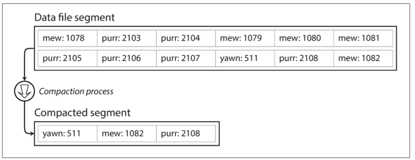
Figure 3-2. Compacting a key-value update log and keeping only the latest value for each key.

Segments can also be merged in the background. Since old segments are immutable, reads and writes can continue while new compacted segments are built.

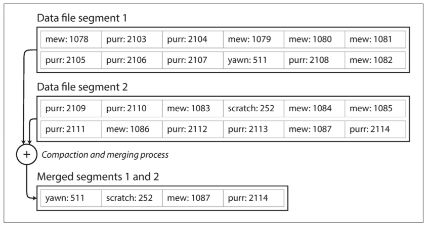
Figure 3-3. Compaction and segment merging at the same time.

Practical implementations need to handle file formats, deletion records called tombstones, crash recovery, partially written records, checksums, and concurrency. Append-only logs are attractive because sequential writes are usually fast, immutable segments simplify recovery, and merging avoids long-term fragmentation.

Hash indexes have two important limits. They must keep keys in memory, and they are inefficient for range queries because every key has to be looked up separately.

SSTables and LSM Trees

An SSTable, or Sorted String Table, stores key-value pairs sorted by key. Each key appears once per merged segment. Sorting enables efficient merging, sparse in-memory indexes, and compressed blocks.

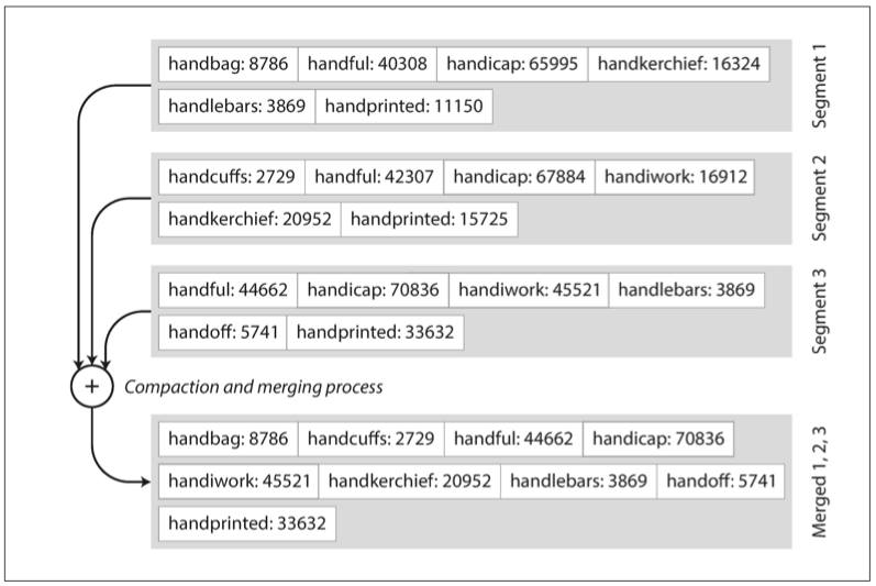
Figure 3-4. Merging several SSTable segments and keeping the newest value for each key.

Because keys are sorted, a sparse index is enough. If a requested key lies between two indexed keys, the engine scans the small block between them.

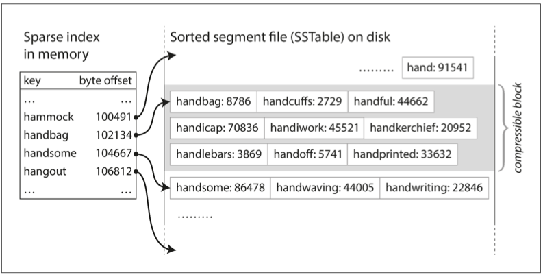
Figure 3-5. An SSTable with an in-memory index.

Writes are first inserted into an in-memory balanced tree called a memtable. When the memtable reaches a threshold, it is written to disk as an SSTable. Reads check the memtable, then the newest segment, then older segments. Background compaction merges segments and removes overwritten or deleted values.

This family of techniques is known as LSM trees. Systems such as LevelDB, RocksDB, Cassandra, HBase, Lucene, Elasticsearch, and Solr use related designs. Bloom filters are often used to avoid unnecessary disk reads for keys that do not exist.

B-Trees

B-trees are the most widely used indexing structure in relational databases. They split data into fixed-size pages, normally around 4 KB, and maintain references from parent pages to child pages.

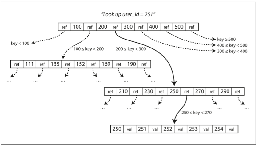
Figure 3-6. Looking up a key using a B-tree index.

To update a value, the database finds the leaf page and modifies it. If the page is full, it is split and the parent page is updated. B-trees keep the tree balanced, so lookups are efficient even for large datasets.

Updates overwrite pages in place, which makes crash recovery harder. Many databases use a write-ahead log so that interrupted operations can be replayed. Concurrency also requires careful latching so readers do not observe an inconsistent tree.

B-Trees Compared With LSM Trees

LSM trees usually provide higher write throughput because they turn random writes into sequential writes and compact data in the background. They can compress well and avoid fragmentation, but compaction can compete with foreground reads and writes, and a key may exist in several segments until compaction finishes.

B-trees are often better for read-heavy workloads because a key is found in one well-defined place. They also make transaction isolation easier because the same key maps to the same index location.

There is no universally superior structure. The right choice depends on workload, hardware, compaction behavior, and latency requirements.

Other Indexing Structures

Primary indexes identify rows, but secondary indexes allow lookup by other fields. Secondary indexes are essential for joins and search conditions. They may point directly to rows or store matching row identifiers.

Indexes can also store values together with keys, a technique called a covering index. Multi-column indexes support queries over several fields. Specialized structures support full-text search, fuzzy matching, geospatial lookup, and multidimensional queries.

Full-text search engines often tolerate spelling differences and rank results by relevance. Geospatial indexes need to search two-dimensional or multidimensional ranges, using structures such as R-trees or space-filling curves.

Keeping Everything in Memory

As memory becomes cheaper, some databases keep most or all data in RAM. In-memory databases can be faster, but their durability still depends on logs, snapshots, replication, or disk-backed recovery. The main advantage is often not avoiding disk I/O, but using data structures that do not need to be encoded as disk pages.

Transaction Processing and Analytics

Online transaction processing (OLTP) systems support user-facing reads and writes with low latency. Online analytical processing (OLAP) systems support complex scans and aggregations over large datasets.

Analytics workloads often use a data warehouse, where data from OLTP systems is periodically extracted, transformed, and loaded. This lets analysts run expensive queries without affecting production transaction systems.

Stars, Snowflakes, and Column Storage

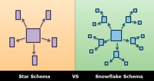
Data warehouses often use star schemas: a large fact table at the center, surrounded by dimension tables. Snowflake schemas normalize dimensions further into sub-dimensions.

Analytical queries frequently scan only a few columns across many rows. Column-oriented storage stores each column together, which reduces I/O and compresses well because values in the same column tend to be similar.

Column compression, bitmap encoding, vectorized processing, and CPU cache-friendly layouts can greatly improve analytical query performance.

Materialized Views and Data Cubes

Materialized views precompute query results and store them for reuse. A data cube is a materialized aggregate over several dimensions. Precomputation speeds up common queries but reduces flexibility and adds maintenance cost when source data changes.

Summary

Storage engines balance read performance, write performance, disk layout, memory usage, crash recovery, and query flexibility. Log-structured engines and B-trees make different trade-offs. Analytics systems make another set of trade-offs by organizing data for scans and aggregation rather than point updates.