Developing Stream Processing Applications with Kafka Streams
What Is Stream Processing?
Stream processing refers to an application that processes an event stream whenever data arrives and continues doing so. In the Kafka ecosystem, it is an application that connects to Kafka Broker as a Consumer, runs polling in an infinite loop, and processes data at short intervals whenever it arrives.
Sometimes multiple records are used for aggregation. Typical patterns include dividing aggregation units by fixed periods and updating aggregate results one record at a time, or buffering records and processing them together at regular intervals.
Stateless or Stateful
Stream processing can be broadly divided into stateless and stateful processing.
Stateless processing is processing that completes using only the event record that arrived. A common example is transforming record A into record B and sending it to another topic or another data store.
Stateful processing stores arriving event records or data generated from them for a certain period and combines them to produce results. Common examples include counting events to calculate totals, averages, and histograms, buffering data for efficient batch-like processing, or joining data with other streams and data stores to improve data quality.
Stateful processing requires a separate data store that holds a certain amount of records. This is called a StateStore. There are several important points to consider for StateStores in stream processing, and they are explained later.
State Stores in Stateful Applications
Because stream processing runs whenever data arrives, using any data store means fetching or saving data each time records arrive.
Therefore, low latency is an important requirement. Depending on data volume, even a simple and fast KVS such as Redis can incur network latency and may not be sufficient.
For this reason, stream processing usually keeps a data store locally on each processing node to keep latency low.
Stream processing frameworks such as Kafka Streams and Apache Flink use RocksDB. RocksDB is an embeddable KVS, so each node can run RocksDB locally and maintain low latency.
Keeping data locally on each node also means data can be lost if a node goes down unexpectedly and cannot recover. To avoid this, a node-independent data persistence mechanism is also required. Because network overhead is unavoidable in that structure, some buffering is needed.
Kafka streaming applications can also run in a distributed form across multiple nodes to guarantee scalability. In that case, the partition assignments being processed can change as the number of nodes increases or decreases. As explained earlier, in the same Consumer Group, only one client can process a single partition. When the number of nodes changes, assignments are redistributed, so the application must account for processing targets moving to different nodes. When processing moves to another node, the StateStore data that was kept locally on the previous node must somehow be moved to the newly assigned node. Otherwise, the previously maintained StateStore data cannot be used. For example, an aggregate count could suddenly return to zero when a node is added. To avoid this, a mechanism that relocates StateStores according to processing-node changes is essential.
What Is Kafka Streams?
Kafka Streams is the official stream processing framework provided by the Apache Kafka development project. It is implemented in Java.
As described above, implementing a stateful application requires a fairly complex state-management structure. Kafka Streams simplifies that complexity through its framework. It can also greatly reduce code even for stateless applications, because Consumer polling loops and Producer clients for sending records to other topics can otherwise become complex.
The concepts described here are covered broadly in the Confluent documentation. Refer to it for more detail.
cf. Confluent | Streams Concepts
Key Features
According to the Confluent documentation, whose company plays a major role in Kafka development, Kafka Streams has the following features.
Powerful
- Makes your applications highly scalable, elastic, distributed, fault-tolerant
- Supports exactly-once processing semantics
- Stateful and stateless processing
- Event-time processing with windowing, joins, aggregations
- Supports Kafka Streams Interactive Queries to unify the worlds of streams and databases
- Choose between a declarative, functional API and a lower-level imperative API for maximum control and flexibility
Powerful
- Provides high scalability, elasticity, distribution, and fault tolerance for applications.
- Supports exactly-once processing semantics.
- Supports stateful and stateless processing.
- Supports event-time processing with windows, joins, and aggregations.
- Supports Kafka Streams Interactive Queries to unify streams and databases.
- Allows choosing between a declarative functional API and a lower-level imperative API for greater control and flexibility.
Lightweight
- Low barrier to entry
- Equally viable for small, medium, large, and very large use cases
- Smooth path from local development to large-scale production
- No processing cluster required
- No external dependencies other than Kafka
Lightweight
- Low barrier to adoption.
- Works for small, medium, large, and very large use cases.
- Provides a smooth path from local development to large-scale production.
- Does not require a processing cluster.
- Has no external dependencies other than Kafka.
The most important point among these is probably that Kafka Streams has no external dependencies other than Kafka. Distributed processing frameworks often require a resource manager such as YARN or another data store, but Kafka Streams does not. This greatly lowers the barrier to adoption.
Tutorial Code
To create an application with Kafka Streams, you write code like the following. This is a slightly modified version of an example from the official documentation.
import org.apache.kafka.streams.KafkaStreams;
import org.apache.kafka.streams.kstream.StreamsBuilder;
import org.apache.kafka.streams.processor.Topology;

// Use the builders to define the actual processing topology, e.g. to specify
// from which input topics to read, which stream operations (filter, map, etc.)
// should be called, and so on.  We will cover this in detail in the subsequent
// sections of this Developer Guide.

StreamsBuilder builder = new StreamsBuilder();
builder
    .stream(inputTopic, Consumed.with(stringSerde, stringSerde))
    .peek((k,v) -> logger.info("Observed event: {}", v))
    .mapValues(s -> s.toUpperCase())
    .peek((k,v) -> logger.info("Transformed event: {}", v))
    .to(outputTopic, Produced.with(stringSerde, stringSerde));
Topology topology = builder.build();
//
// OR
//
topology.addProcessor(...); // when using the Processor API

// Use the configuration properties to tell your application where the Kafka cluster is,
// which Serializers/Deserializers to use by default, to specify security settings,
// and so on.
Properties props = ...;

KafkaStreams streams = new KafkaStreams(topology, props);
streams.start(); // non blocking
In this way, Kafka Streams can create Consumers and Producers that connect to Kafka and simplify processing-thread startup simply by chaining DSL calls or implementing Java classes according to the specific Processor API interfaces.
Kafka Streams Application Model
Kafka Streams builds applications by combining Source Nodes, Processor Nodes, and Sink Nodes into a unit called a Topology. The meaning of each component is explained below.
Topology
The word topology is originally a mathematical term. Without going into mathematical detail, it is a field that focuses on the properties of shapes. Derived from that, network topology refers to the structural pattern of a network graph. Kafka Streams Topology can be understood in the same way as network topology.
Kafka Streams operates by connecting nodes with specific roles to build a graph structure and form a Topology. A Topology can be formed from two or more sub-topologies.
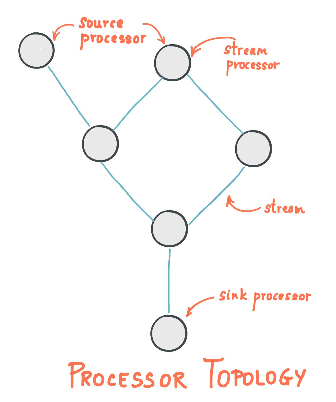
Image: Confluent | Streams Architecture
The Kafka Streams Topology object holds one or more of these graph structures.
Whether two or more sub-topologies are created depends on how the application is defined. If one application receives data from multiple source topics and there is no direct dependency between Processor Nodes or Sink Nodes that depend on those source topics, separate sub-topologies can be created. In the example above, there are multiple Source Nodes, but because the Processor below depends on both Source Nodes, the graph is connected as one. In that case there is one sub-topology. If the Source Node on the left depended only on a Processor Node that was independent from the rest, there could be two sub-topologies.
Source Node
A Source Node performs the processing that receives data from Kafka topics. Kafka Streams has three patterns for receiving data. Details are explained in the DSL section. In the sample code above, stream in the DSL corresponds to this.
Processor Node
A Processor Node actually processes data received from a Source Node. Most of what developers implement belongs to this node. Multiple Processor Nodes can be connected, and splitting processing steps can make the implementation easier to read. In the DSL sample above, peek and mapValues correspond to this.
Sink Node
A Sink Node sends data to another Kafka topic. In the DSL sample above, to corresponds to this.
Kafka Streams applications are built by reading data from a topic with a Source Node, processing it with Processor Nodes, temporarily storing it or saving it to another data store, and if necessary sending it to another topic with a Sink Node to connect it to further processing.
Task
Kafka Streams is designed to perform distributed processing across multiple machines. Kafka Streams assigns processing to clients in units called Tasks, corresponding to the number of partitions in the source topics polled by a sub-topology.
For example, suppose Topology A has sub-topologies A-1 and A-2, where A-1 refers to topic B-1 and A-2 refers to topic B-2. If topic B-1 has 8 partitions and topic B-2 has 10 partitions, tasks 1_0 through 1_7 and 2_0 through 2_9 are created. The total number of tasks is 18. These 18 tasks are assigned to clients in the current Consumer Group. There are several assignment strategies, and their details are covered later.
DSL
Kafka Streams provides a convenient DSL to build the Topology described above. With the DSL, you can write stream applications easily by chaining lambdas through method calls.
For a full overview, refer to the official documentation.
Only important DSL elements are introduced below.
KStream, KTable, GlobalKTable
Kafka Streams DSL provides three patterns for receiving data from topics. The DSL is expressed by chaining method calls on objects representing these three inputs.
KStream
KStream represents a simple input stream from a Kafka topic.
StreamsBuilder builder = new StreamsBuilder();

KStream<String, Long> wordCounts = builder.stream(
    "word-counts-input-topic", /* input topic */
    Consumed.with(
      Serdes.String(), /* key serde */
      Serdes.Long()   /* value serde */
    );
When receiving input, you specify a Serde, which combines Serializer and Deserializer. In actual input, only the Deserializer side is used.
Through this Serde, Kafka Streams automatically converts Java objects and byte arrays.
KTable, GlobalKTable
KTable and GlobalKTable represent input streams that can be treated like tables. Being table-like means that all records entered into Kafka Broker from the beginning of loading to the current point are maintained locally, so they can be joined with other streams or used like a KVS.
This keeps the state of input records, so using KTable is a stateful application.
KTable keeps each partition’s content only on assigned clients, while GlobalKTable keeps all partitions of one topic on every node. Therefore, pay attention to the amount of data in the input topic.
GlobalKTable<String, Long> wordCounts = builder.globalTable(
    "word-counts-input-topic",
    Materialized.<String, Long, KeyValueStore<Bytes, byte[]>>as(
      "word-counts-global-store" /* table/store name */)
      .withKeySerde(Serdes.String()) /* key serde */
      .withValueSerde(Serdes.Long()) /* value serde */
    );
KTable requires a store name and Serdes for the data to store. Using this store name, a RocksDB database file is created on each node and data is accumulated there. This data store is called a StateStore. With methods such as Materialized.as in the example above, you can switch the store name or Serdes, or pass other arguments to use an in-memory data store.
Data stored in a StateStore remains after process restart unless the store is in-memory. However, when partition assignment changes and the responsible Task changes, the data may become unnecessary or need to be rebuilt. RocksDB data that is no longer needed is automatically deleted after a certain period.
GroupBy, GroupByKey
These DSL operations specify which key should be used when aggregating a KStream or KTable. They must be called before count or aggregate.
KGroupedStream<String, String> groupedStream = stream.groupBy(
    (key, value) -> value,
    Grouped.with(
      Serdes.String(), /* key (note: type was modified) */
      Serdes.String())  /* value */
  );
Using groupBy always causes repartitioning. Repartitioning automatically creates a topic for repartitioning, sends records to that topic, and reads them again. Because this creates duplicate network and storage load, repartitioning should be avoided as much as possible.
To avoid repartitioning, use groupByKey.
KGroupedStream<String, String> groupedStream = stream.groupByKey(
    Grouped.with(
      Serdes.String, /* key */
      Serdes.String())     /* value */
  );
groupByKey groups by using the current key as-is. If the key has not changed during processing, repartitioning is not performed. If the key has changed through transformations such as map, repartitioning will still occur even when groupByKey is used.
aggregate
aggregate is the most general-purpose DSL operation for implementing aggregation. It receives three lambdas: an initializer that creates the initial value, an adder that runs when a new record arrives, and an optional subtractor that uses information from the old record.
KTable<byte[], Long> aggregatedTable = groupedTable.aggregate(
    () -> 0L, /* initializer */
    (aggKey, newValue, aggValue) -> aggValue + newValue.length(), /* adder */
    (aggKey, oldValue, aggValue) -> aggValue - oldValue.length(), /* subtractor */
    Materialized.as("aggregated-table-store") /* state store name */
    .withValueSerde(Serdes.Long()) /* serde for aggregate value */
);
If aggregation results are not continuously stored locally on the processing node, the current aggregate value cannot be known when the next record arrives. Therefore, aggregation processing necessarily requires a KTable. Aggregated results are saved and maintained in the StateStore automatically built by the DSL.
There are several important details about StateStores, so they are explained later. For now, remember that results are stored in a place called a StateStore.
windowedBy
windowedBy is a DSL operation that divides the aggregation range by fixed time periods. It can be used to keep calculating totals every five minutes or count events included in one session. Window processing depends on the time axis, so record timestamps and retention periods are important. Old timestamp records may arrive late, and if old aggregation data is kept indefinitely, data grows without limit and pressures storage. To handle this, window processing allows a separate retention period to be set.
// Aggregating with time-based windowing (here: with 5-minute tumbling windows)
KTable<Windowed<String>, Long> timeWindowedAggregatedStream = groupedStream.windowedBy(TimeWindows.of(Duration.ofMinutes(5)))
    .aggregate(
      () -> 0L, /* initializer */
      (aggKey, newValue, aggValue) -> aggValue + newValue, /* adder */
      Materialized.<String, Long, WindowStore<Bytes, byte[]>>as("time-windowed-aggregated-stream-store") /* state store name */
        .withValueSerde(Serdes.Long())); /* serde for aggregate value */
There are currently four window types: Tumbling Window, Sliding Window, Hopping Window, and Session Window. Because this is relatively complex, refer to the Confluent documentation for details.
Processor API
The Processor API is the low-level API of Kafka Streams. All of the DSL operations above are implemented with this Processor API.
Simply put, the Processor API can be used by defining classes. The init method receives a ProcessorContext object, which can be used to obtain Kafka Streams information, refer to StateStores, and forward data to subsequent processing. Refer to the Confluent documentation for details.
The actual processing is implemented in the process method, which is called whenever a record arrives. You can also schedule processing at fixed intervals. The ProcessorContext#schedule method registers a Punctuator that runs automatically at fixed intervals. Kafka Streams provides two timestamp modes for scheduling intervals: STREAM_TIME and WALL_CLOCK_TIME. See the linked documentation above for the difference.
The following code sample is quoted from that documentation. The important parts are getting the StateStore, registering scheduled processing, and calling context.forward to pass records to the next step.
public class WordCountProcessor implements Processor<String, String, String, String> {
    private KeyValueStore<String, Integer> kvStore;

    @Override
    public void init(final ProcessorContext<String, String> context) {
        context.schedule(Duration.ofSeconds(1), PunctuationType.STREAM_TIME, timestamp -> {
            try (final KeyValueIterator<String, Integer> iter = kvStore.all()) {
                while (iter.hasNext()) {
                    final KeyValue<String, Integer> entry = iter.next();
                    context.forward(new Record<>(entry.key, entry.value.toString(), timestamp));
                }
            }
        });
        kvStore = context.getStateStore("Counts");
    }

    @Override
    public void process(final Record<String, String> record) {
        final String[] words = record.value().toLowerCase(Locale.getDefault()).split("\\W+");

        for (final String word : words) {
            final Integer oldValue = kvStore.get(word);

            if (oldValue == null) {
                kvStore.put(word, 1);
            } else {
                kvStore.put(word, oldValue + 1);
            }
        }
    }

    @Override
    public void close() {
        // close any resources managed by this processor
        // Note: Do not close any StateStores as these are managed by the library
    }
}
To include this in Kafka Streams, create a Topology directly or call Topology#addProcessor on a topology generated by StreamsBuilder#build to register the Processor class. If the Processor uses a StateStore, pass the store name and associate it. Otherwise the Processor API cannot find the StateStore and an exception occurs.
Topology builder = new Topology();

// add the source processor node that takes Kafka topic "source-topic" as input
builder.addSource("Source", "source-topic")

    // add the WordCountProcessor node which takes the source processor as its upstream processor
    .addProcessor("Process", () -> new WordCountProcessor(), "Source")

    // add the count store associated with the WordCountProcessor processor
    .addStateStore(countStoreSupplier, "Process")

    // add the sink processor node that takes Kafka topic "sink-topic" as output
    // and the WordCountProcessor node as its upstream processor
    .addSink("Sink", "sink-topic", "Process");
What StateStore Actually Is
Official StateStores are broadly divided into two types: persistent stores using RocksDB and volatile in-memory stores that disappear when the process exits. Persistent stores are probably the most commonly used. First, let us look at common elements. If you implement the API yourself, you can also define a custom StateStore.
When using a StateStore from the low-level API, you can build the StateStore yourself.
// Creating a persistent key-value store:
// here, we create a `KeyValueStore<String, Long>` named "persistent-counts".
import org.apache.kafka.streams.processor.StateStoreSupplier;
import org.apache.kafka.streams.state.StoreBuilder;
import org.apache.kafka.streams.state.Stores;

StoreBuilder countStoreBuilder =
  Stores.keyValueStoreBuilder(
    Stores.persistentKeyValueStore("persistent-counts"),
    Serdes.String(),
    Serdes.Long()
  );
To use it through the Processor API, use it in the following form.
KeyValueStore<String, Long> counterStore = context.getStateStore("persistent-counts");
long count = counterStore.fetch("key");
count++;
counterStore.put("key", count);
This example fetches a value by exact key match, but StateStores provided by Kafka Streams are sorted by key bytes, so you can also use the range method to obtain keys in a certain range.
Important StateStore properties are as follows.
- It is a KVS and is sorted by key.
- The actually stored key and value are byte arrays, and Serialize/Deserialize is performed when interacting with the application.
- Durability is guaranteed by a changelog topic.
- It has a cache mechanism for reads and writes.
Changelog Topics
As mentioned briefly earlier, when a StateStore is used, a changelog topic is automatically created in Kafka Broker. It is disabled by default for in-memory stores.
A changelog topic is a topic that holds changes written to the StateStore. Whenever data is written to or deleted from the StateStore, such as by writing null, a record is sent to the changelog topic.
Kafka Streams uses this changelog topic to handle processing node failures and task reassignment.
When a Kafka Streams process starts, if the application is defined to use a StateStore and the local store has no StateStore data, Kafka Streams performs restore processing. It reads all records from the changelog topic in Kafka Broker and restores the local StateStore.
Similarly, when rebalancing occurs due to node increases or decreases and tasks are reassigned, if a StateStore corresponding to a newly assigned task ID does not exist locally, restore processing runs first and then processing continues.
In production, Kafka Broker is usually configured with three or more replicas, so fault tolerance for the data itself is guaranteed by Kafka Broker’s functionality.
Notes on Restore Processing
The most important thing to watch when using StateStores is restore processing.
Kafka Streams stops processing when restore is required. Processing starts or resumes only after restore processing completes. That means if the amount of data accumulated in StateStore becomes very large, restore can take a long time, and when a node goes down or the number of nodes changes, processing may stop for a long period.
Avoiding this is currently a difficult problem. In practice, you need a mechanism that reduces the amount of data, for example by accepting network overhead and moving old or rarely used data to external storage.
Disabling Changelog
When creating a StateStore, calling withLoggingDisabled() on StoreBuilder disables the relationship with the changelog. For in-memory stores, it is disabled by default.
If the changelog topic cannot be used, restore processing is not performed. When using a RocksDB store, data remains as long as a task with the same ID runs on the same node. However, if tasks are redistributed by Consumer rebalancing or the processing node goes down and cannot recover, that data disappears.
The main use case is a local cache. Even when the amount is too large for memory, the file system can be used as node-local cache.
For example, immutable data can be accumulated in an external data store. The first access incurs network overhead, but afterward it can be cached in the local file system and accessed without going through the network.
StateStore Cache
Because of the nature of stream processing, the same key may be read and written many times in a short period. For example, when calculating counts by user_id, records for that user may arrive in bursts. In such a situation, writing to storage and updating the changelog topic every time can create unnecessary overhead.
Kafka Streams enables caching by default to avoid this. Written content is kept in memory for a certain period, and at flush timing it is written to the actual StateStore and the changelog is updated.
In KTable built with the DSL, this cache delays forwarding. For example, when aggregate results are used by the next DSL operation or sent to another topic, the default behavior buffers them in the StateStore cache for a certain period. When a certain time passes or cache memory is consumed, CacheFlushListener forwards the record to the next processor.
What WindowStore Actually Is
The DSL section introduced windowedBy. This DSL allows records to be aggregated for each fixed time window.
In fact, this is implemented by a StateStore variant called WindowStore. A WindowStore is created as follows. This example creates a WindowStore that retains two hours of data with one-minute windows.
StoreBuilder<WindowStore<String, Long>> counterStoreByMinute =
      Stores.windowStoreBuilder(
              Stores.persistentWindowStore(
                  "counter",
                  Duration.ofHours(2),
                  Duration.ofMinutes(1),
                  false),
              Serdes.String(),
              Serdes.Long());
To use it through the Processor API, use it as follows.
WindowStore<String, Long> counterStoreByMinute = context.getStateStore("counter");
long durationMillis = Duration.ofMinutes(1).toMillis();
long currentWindowStart = (context.timestamp() / durationMillis) * durationMillis;
long count = counterStoreByMinute.fetch("key", windowStart);
count++;
counterStoreByMinute.put("key", count, currentWindowStart);
Values are fetched and stored by assigning timestamps to keys and values. When used behind the DSL, Kafka Streams automatically sets the Time Window from the timestamp. When handling WindowStore directly, you must manually calculate which timestamp is the start of the TimeWindow. The Window Duration given to the WindowStore is used to determine the width of the window based on the recorded timestamp.
The example above is simple, but you can also pass start and end timestamps and retrieve records in that range in order. As with a normal KeyValueStore, key range searches can also be combined with timestamp start and end range searches.
Internally, WindowStore consists of multiple RocksDB stores and is divided into approximate segments by recorded timestamp. When saving, the segment is identified from the timestamp and data is written to that area. When fetching, data is retrieved only from the segments in the target range, reducing the search range. Because the segment can be determined from the timestamp range, data past the retention period compared with the currently processed timestamp can be discarded simply by deleting whole files.
When writing, a millisecond Unix timestamp is automatically appended to the end of the record key, such as the string "key" in the example above, and the result is recorded.